The principle of PID is very simple. Three subsets (P, I, D) of one equation that each have their own task. Nevertheless, the PID formula in your DCS/PLC can have many forms. The most common equations are the series and parallel equation. In this blog we'll show you that it's extremely important to know the different formulas to tune your controller.
When you look in the manuals of the DCS/PLC systems on the markets, you will see many variants of these 2 equations below. The word variants might suggest that the differences are not that important. But that's not true. All these variants have different functionalities and can achieve different closed-loop behaviour.
Series/interacting:

Parallel:

Non-interacting:

Why are there so many variants? Some of them are coming from the time of pneumatic and analog electronic control. Some equations were easy to implement with resistors and capacitors in analog PID controllers.
That limitation dictated the equation type. Companies kept the tradition they were used to. Mergers and acquisitions of companies resulted in brands with different DCS systems and therefore different equations.

Different PID equations: different functionalities
The generic PID tuning formula is shown below.
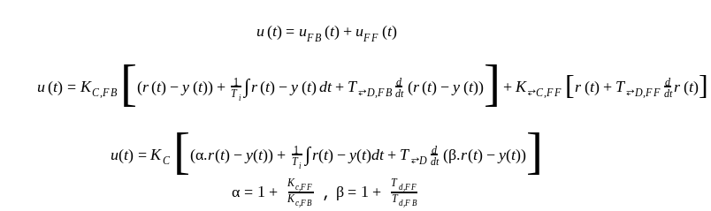
It contains feedforward action, the possibility to allow the D action to work on the error or on the PV only, double derivates (for mechatronics), and so on. Here is what you need to know:
- It is a no brainer that the I action can only work on the error (R-Y).
- The alpha parameters is a feedforward action. Traditionally the P action works on the error. But it can also act differently on the PV and the SP. In that case some part of the setpoint signal can directly be send to the output of the controller.
- The D action can act on the Error (R-Y) or on the PV only (0.R-Y) or on a combination of both.
- Some DCS systems apply a fixed filter on the D action, others use a filter that can be tuned.
An example of 2 PID formulas used in Foxboro DCS is shown below.
Formula 1 : PID function of an PIDA MODOPT = 6 (Non-interacting PID)

Formula 1: PID function of an PIDA MODOPT = 5 (Interacting PID)
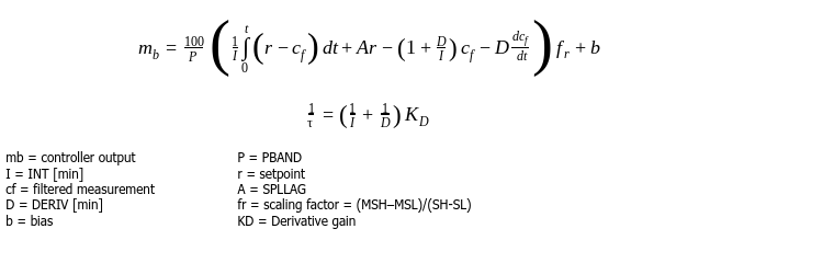
Most functionalities mentioned above are available, provided the right parameters are set or selected. Nevertheless, the formula itself “looks” completely different. Why make it so complicated? Why not embrace the KISS (Keep it Simple) approach? Here are some reasons:
- Applying D action on the PV only, instead of the error: This will allow having the stabilizing effect of the D action, without the big output kick when the setpoint changes.
- A feedforward action: Without Feedforward a PID controller can only be tuned for optimal setpoint tracking OR for optimal disturbance rejection. It is one or the other. For example, you tune for optimal setpoint tracking and you will have to live with the closed-loop disturbance rejection behavior that you will get (or visa versa). With Feedforward you can tune for optimal setpoint tracking AND for optimal disturbance rejection. Much more performance if you should just know how to parameterize this feedforward parameter.
So, selecting the right formula and the right functionality is key when selecting the PID algorithm in your DCS.
Different PID equations: different tuning
After having selected the right equation the tuning can start. The format of the selected equation has a huge effect on the tuning. The most simple example is the use of a Gain or proportional band (PB) to tune the P action of the PID.
The relation between the Gain and the Proportional band is simple. Gain = (100 x Scaling)/PB. Assume the scaling equals 1. So, if you computed a Gain of 2 it is important to know if the DCS equation uses the Gain or PB parameter. In the second case, not 2 but 50 has to be entered as the tuning parameter. The difference is a factor of 25! Your loop can easily become unstable when this simple knowledge is not applied when entering the new tuning parameters.
When tuning with for example Ziegler Nichols, it is assumed that you use a certain equation type. The resulting parameters are only for that equation. When using others the parameters have to be translated to the targeted DCS. Only a detailed study of the manual will reveal how to do it.
Keep it simple: use tuning software
An easier way to handle all these equations and functionalities is to use tuning software where all that knowledge is built in. Libraries of all common DCS/PLC systems are available. Just select the hardware that you have and all results will be presented such that you can copy them without any risk to your DCS/PLC.
You save a lot of time and avoid sweating hands when you have to enter the numbers.
Another advantage is that tuning software will also compute the optimal Feedforward parameters, filter parameters for D, and so on. Most ruled based tuning methods do not take these “exotic” parameters into account. Tuning these extra parameters after the rule-based tuning is not a good idea. You need to optimize them all together.
Tools like INCA PID Tuner and INCA AptiTune have all the functionalities built-in for risk-free and optimal tuning. We would love to offer you a free, and no-obligation live demo of INCATools AptiTune. So we can show you all the possiobilities tailored to your situation.